Modelling shading losses in modules with bypass diodes

This example illustrates how to use the loss model proposed by Martinez et al. [1]. The model proposes a power output losses factor by adjusting the incident direct and circumsolar beam irradiance fraction of a PV module based on the number of shaded blocks. A block is defined as a group of cells protected by a bypass diode. More information on blocks can be found in the original paper [1] and in the pvlib.shading.direct_martinez() documentation.

The following key functions are used in this example:

1. pvlib.shading.direct_martinez() to calculate the power output losses fraction due to shading.

2. pvlib.shading.shaded_fraction1d() to calculate the fraction of shaded surface and consequently the number of shaded blocks due to row-to-row shading.

3. pvlib.tracking.singleaxis() to calculate the rotation angle of the trackers.

Problem description

Let’s consider a PV system with the following characteristics:

• Two north-south single-axis trackers, each one having 6 modules.

• The rows have the same true-tracking tilt angles. True tracking is chosen in this example, so shading is significant.

• Terrain slope is 7 degrees downward to the east.

• Row axes are horizontal.

• The modules are comprised of multiple cells. We will compare these cases:

  • modules with one bypass diode

  • modules with three bypass diodes

  • half-cut cell modules with three bypass diodes in portrait and landscape

Setting up the system

Let’s start by defining the system characteristics, location and the time range for the analysis.

import pvlib
import pandas as pd
import numpy as np
import matplotlib.pyplot as plt
from matplotlib.dates import DateFormatter

pitch = 4  # meters
width = 1.5  # meters
gcr = width / pitch  # ground coverage ratio
N_modules_per_row = 6
axis_azimuth = 180  # N-S axis
axis_tilt = 0  # flat because the axis is perpendicular to the slope
cross_axis_tilt = -7  # 7 degrees downward to the east

latitude, longitude = 40.2712, -3.7277
locus = pvlib.location.Location(
    latitude,
    longitude,
    tz="Europe/Madrid",
    altitude=pvlib.location.lookup_altitude(latitude, longitude),
)

times = pd.date_range("2001-04-11T04", "2001-04-11T20", freq="10min")

True-tracking algorithm and shaded fraction

Since this model is about row-to-row shading, we will use the true-tracking algorithm to calculate the trackers rotation. Back-tracking eliminates shading between rows, and since this example is about shading, we will not use it.

Then, the next step is to calculate the fraction of shaded surface. This is done using pvlib.shading.shaded_fraction1d(). Using this function is straightforward with the variables we already have defined. Then, we can calculate the number of shaded blocks by rounding up the shaded fraction by the number of blocks along the shaded length.

# Calculate solar position to get single-axis tracker rotation and irradiance
solar_pos = locus.get_solarposition(times)
solar_apparent_zenith, solar_azimuth = (
    solar_pos["apparent_zenith"],
    solar_pos["azimuth"],
)  # unpack for better readability

tracking_result = pvlib.tracking.singleaxis(
    apparent_zenith=solar_apparent_zenith,
    apparent_azimuth=solar_azimuth,
    axis_tilt=axis_tilt,
    axis_azimuth=axis_azimuth,
    max_angle=(-90 + cross_axis_tilt, 90 + cross_axis_tilt),  # (min, max)
    backtrack=False,
    gcr=gcr,
    cross_axis_tilt=cross_axis_tilt,
)

tracker_theta, aoi, surface_tilt, surface_azimuth = (
    tracking_result["tracker_theta"],
    tracking_result["aoi"],
    tracking_result["surface_tilt"],
    tracking_result["surface_azimuth"],
)  # unpack for better readability

# Calculate the shade fraction
shaded_fraction = pvlib.shading.shaded_fraction1d(
    solar_apparent_zenith,
    solar_azimuth,
    axis_azimuth,
    axis_tilt=axis_tilt,
    shaded_row_rotation=tracker_theta,
    shading_row_rotation=tracker_theta,
    collector_width=width,
    pitch=pitch,
    cross_axis_slope=cross_axis_tilt,
)

Number of shaded blocks

The number of shaded blocks depends on the module configuration and number of bypass diodes. For example, modules with one bypass diode will behave like one block. On the other hand, modules with three bypass diodes will have three blocks, except for the half-cut cell modules, which will have six blocks; 2x3 blocks where the two rows are along the longest side of the module. We can argue that the dimensions of the system change when you switch from portrait to landscape, but for this example, we will consider it the same.

The number of shaded blocks is calculated by rounding up the shaded fraction by the number of blocks along the shaded length. So let’s define the number of blocks for each module configuration:

• 1 bypass diode: 1 block

• 3 bypass diodes: 3 blocks in landscape; 1 in portrait

• 3 bypass diodes half-cut cells: - 2 blocks in portrait - 3 blocks in landscape

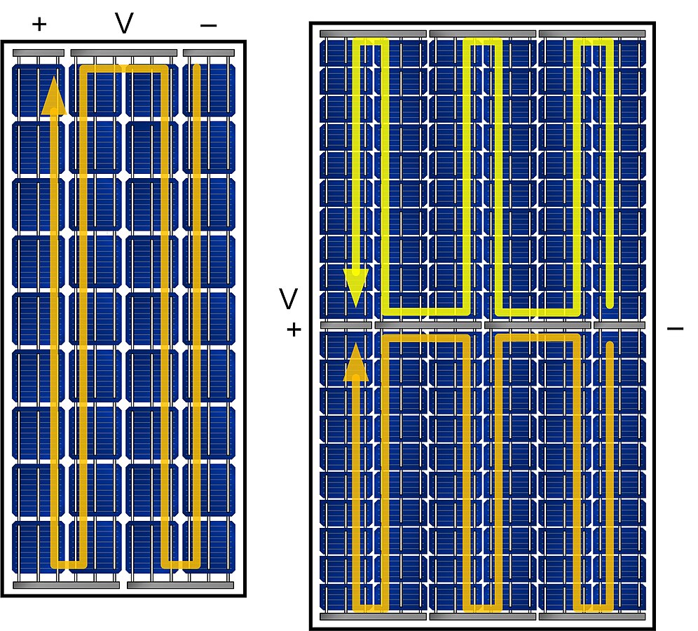
Left: common module layout. Right: half-cut cells module layout. Each module has three bypass diodes. On the left, they connect cell columns 1-2, 2-3 & 3-4. On the right, they connect cell columns 1-2, 3-4 & 5-6. Source: César Domínguez. CC BY-SA 4.0, Wikimedia Commons

In the image above, each orange U-shaped string section is a block. By symmetry, the yellow inverted-U’s of the subcircuit are also blocks. For this reason, the half-cut cell modules have 6 blocks in total: two along the longest side and three along the shortest side.

blocks_per_module = {
    "1 bypass diode": 1,
    "3 bypass diodes": 3,
    "3 bypass diodes half-cut, portrait": 2,
    "3 bypass diodes half-cut, landscape": 3,
}

# Calculate the number of shaded blocks during the day
shaded_blocks_per_module = {
    k: np.ceil(blocks_N * shaded_fraction)
    for k, blocks_N in blocks_per_module.items()
}

Plane of array irradiance example data

To calculate the power output losses due to shading, we need the plane of array irradiance. For this example, we will use synthetic data:

clearsky = locus.get_clearsky(
    times, solar_position=solar_pos, model="ineichen"
)
dni_extra = pvlib.irradiance.get_extra_radiation(times)
airmass = pvlib.atmosphere.get_relative_airmass(solar_apparent_zenith)
sky_diffuse = pvlib.irradiance.perez_driesse(
    surface_tilt, surface_azimuth, clearsky["dhi"], clearsky["dni"],
    solar_apparent_zenith, solar_azimuth, dni_extra, airmass,
)  # fmt: skip
poa_components = pvlib.irradiance.poa_components(
    aoi, clearsky["dni"], sky_diffuse, poa_ground_diffuse=0
)  # ignore ground diffuse for brevity
poa_global, poa_direct = (
    poa_components["poa_global"],
    poa_components["poa_direct"],
)

Results

Now that we have the number of shaded blocks for each module configuration, we can apply the model and estimate the power loss due to shading.

Note that this model is not linear with the shaded blocks ratio, so there is a difference between applying it to just a module or a whole row.

shade_losses_per_module = {
    k: pvlib.shading.direct_martinez(
        poa_global=poa_global,
        poa_direct=poa_direct,
        shaded_fraction=shaded_fraction,
        shaded_blocks=module_shaded_blocks,
        total_blocks=blocks_per_module[k],
    )
    for k, module_shaded_blocks in shaded_blocks_per_module.items()
}

shade_losses_per_row = {
    k: pvlib.shading.direct_martinez(
        poa_global=poa_global,
        poa_direct=poa_direct,
        shaded_fraction=shaded_fraction,
        shaded_blocks=module_shaded_blocks * N_modules_per_row,
        total_blocks=blocks_per_module[k] * N_modules_per_row,
    )
    for k, module_shaded_blocks in shaded_blocks_per_module.items()
}

Plotting the results

fig, (ax1, ax2) = plt.subplots(2, 1, sharex=True)
fig.suptitle("Martinez power losses due to shading")
for k, shade_losses in shade_losses_per_module.items():
    linestyle = "--" if k == "3 bypass diodes half-cut, landscape" else "-"
    ax1.plot(times, shade_losses, label=k, linestyle=linestyle)
ax1.legend(loc="upper center")
ax1.grid()
ax1.set_ylabel(r"$P_{out}$ losses")
ax1.set_title("Per module")

for k, shade_losses in shade_losses_per_row.items():
    linestyle = "--" if k == "3 bypass diodes half-cut, landscape" else "-"
    ax2.plot(times, shade_losses, label=k, linestyle=linestyle)
ax2.legend(loc="upper center")
ax2.grid()
ax2.set_xlabel("Time")
ax2.xaxis.set_major_formatter(DateFormatter("%H:%M", tz="Europe/Madrid"))
ax2.set_ylabel(r"$P_{out}$ losses")
ax2.set_title("Per row")
fig.tight_layout()
fig.show()

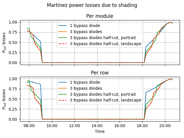
Note how the half-cut cell module in portrait performs better than the normal module with three bypass diodes. This is because the number of shaded blocks is less along the shaded length is higher in the half-cut module. This is the reason why half-cut cell modules are preferred in portrait orientation.

References

[1] (1,2)

F. Martínez-Moreno, J. Muñoz, and E. Lorenzo, ‘Experimental model to estimate shading losses on PV arrays’, Solar Energy Materials and Solar Cells, vol. 94, no. 12, pp. 2298-2303, Dec. 2010, DOI: 10.1016/j.solmat.2010.07.029.