Note
Go to the end to download the full example code.
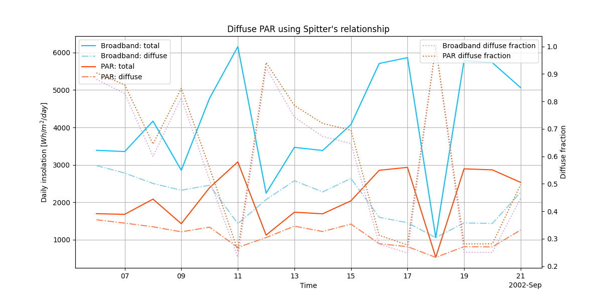
Calculating daily diffuse PAR using Spitter’s relationship#
This example demonstrates how to calculate the diffuse photosynthetically active radiation (PAR) from diffuse fraction of broadband insolation.
The photosynthetically active radiation (PAR) is a key metric in quantifying
the photosynthesis process of plants. As with broadband irradiance, PAR can
be divided into direct and diffuse components. The diffuse fraction of PAR
with respect to the total PAR is important in agrivoltaic systems, where
crops are grown under solar panels. The diffuse fraction of PAR can be
calculated using the Spitter’s relationship [1] implemented in
diffuse_par_spitters().
This model requires the average daily solar zenith angle and the
daily fraction of the broadband insolation that is diffuse as inputs.
Note
Understanding the distinction between the broadband insolation and the PAR is a key concept. Broadband insolation is the total amount of solar energy that gets to a surface, often used in PV applications, while PAR is a measurement of a narrower spectrum of wavelengths that are involved in photosynthesis. See section on Photosynthetically Active insolation in pp. 222-223 of [1].
References#
Read some example data#
Let’s read some weather data from a TMY3 file and calculate the solar position.
import pvlib
import pandas as pd
import matplotlib.pyplot as plt
from matplotlib.dates import AutoDateLocator, ConciseDateFormatter
from pathlib import Path

# Datafile found in the pvlib distribution
DATA_FILE = Path(pvlib.__path__[0]).joinpath("data", "723170TYA.CSV")

tmy, metadata = pvlib.iotools.read_tmy3(
    DATA_FILE, coerce_year=2002, map_variables=True
)
tmy = tmy.filter(
    ["ghi", "dhi", "dni", "pressure", "temp_air"]
)  # remaining columns are not needed
tmy = tmy["2002-09-06":"2002-09-21"]  # select some days

solar_position = pvlib.solarposition.get_solarposition(
    # TMY timestamp is at end of hour, so shift to center of interval
    tmy.index.shift(freq="-30T"),
    latitude=metadata["latitude"],
    longitude=metadata["longitude"],
    altitude=metadata["altitude"],
    pressure=tmy["pressure"] * 100,  # convert from millibar to Pa
    temperature=tmy["temp_air"],
)
solar_position.index = tmy.index  # reset index to end of the hour
/home/docs/checkouts/readthedocs.org/user_builds/pvlib-python/checkouts/2447/docs/examples/agrivoltaics/plot_diffuse_PAR_Spitters_relationship.py:60: FutureWarning: 'T' is deprecated and will be removed in a future version, please use 'min' instead.
  tmy.index.shift(freq="-30T"),
Calculate daily values#
The daily average solar zenith angle and the daily diffuse fraction of broadband insolation are calculated as follows:
daily_solar_zenith = solar_position["zenith"].resample("D").mean()
# integration over the day with a time step of 1 hour
daily_tmy = tmy[["ghi", "dhi"]].resample("D").sum() * 1
daily_tmy["diffuse_fraction"] = daily_tmy["dhi"] / daily_tmy["ghi"]
Calculate Photosynthetically Active Radiation#
The total PAR can be approximated as 0.50 times the broadband horizontal insolation (integral of GHI) for an average solar elevation higher that 10°. See section on Photosynthetically Active Radiation in pp. 222-223 of [1].
par = pd.DataFrame({"total": 0.50 * daily_tmy["ghi"]}, index=daily_tmy.index)
if daily_solar_zenith.min() < 10:
    raise ValueError(
        "The total PAR can't be assumed to be half the broadband insolation "
        + "for average zenith angles lower than 10°."
    )

# Calculate broadband insolation diffuse fraction, input of the Spitter's model
daily_tmy["diffuse_fraction"] = daily_tmy["dhi"] / daily_tmy["ghi"]

# Calculate diffuse PAR fraction using Spitter's relationship
par["diffuse_fraction"] = pvlib.irradiance.diffuse_par_spitters(
    solar_position["zenith"], daily_tmy["diffuse_fraction"]
)

# Finally, calculate the diffuse PAR
par["diffuse"] = par["total"] * par["diffuse_fraction"]
Plot the results#
Insolation on left axis, diffuse fraction on right axis
fig, ax_l = plt.subplots(figsize=(12, 6))
ax_l.set(
    xlabel="Time",
    ylabel="Daily insolation $[Wh/m^2/day]$",
    title="Diffuse PAR using Spitter's relationship",
)
ax_l.xaxis.set_major_formatter(
    ConciseDateFormatter(AutoDateLocator(), tz=daily_tmy.index.tz)
)
ax_l.plot(
    daily_tmy.index,
    daily_tmy["ghi"],
    label="Broadband: total",
    color="deepskyblue",
)
ax_l.plot(
    daily_tmy.index,
    daily_tmy["dhi"],
    label="Broadband: diffuse",
    color="skyblue",
    linestyle="-.",
)
ax_l.plot(daily_tmy.index, par["total"], label="PAR: total", color="orangered")
ax_l.plot(
    daily_tmy.index,
    par["diffuse"],
    label="PAR: diffuse",
    color="coral",
    linestyle="-.",
)
ax_l.grid()
ax_l.legend(loc="upper left")

ax_r = ax_l.twinx()
ax_r.set(ylabel="Diffuse fraction")
ax_r.plot(
    daily_tmy.index,
    daily_tmy["diffuse_fraction"],
    label="Broadband diffuse fraction",
    color="plum",
    linestyle=":",
)
ax_r.plot(
    daily_tmy.index,
    par["diffuse_fraction"],
    label="PAR diffuse fraction",
    color="chocolate",
    linestyle=":",
)
ax_r.legend(loc="upper right")

plt.show()
Total running time of the script: (0 minutes 0.287 seconds)